Introduction to Algorithm Analysis (5): HeapSort

Last time we branched out from just algorithms and began analyzing a very simple data structure and operations on it. This time around we will come full circle, by first introducing one more simple data structure - the heap - and then utilizing it to derive and implement yet another comparison based sorting algorithm, our first exhibiting provably optimal worst case complexity: HeapSort!

As usual, let's first step back and define what we are working with.

What is a heap?

The term itself tends to be the cause of some confusion, as it is unfortunately overloaded in our field, used for at least two distinct things.

Especially those of our readers well versed in a language with manual memory management might know the area in which dynamic memory is allocated - the free store - is frequently referred to as the heap. Whilst also quite fascinating and relevant for real life performance of many data structures and algorithms, it is entirely unrelated to the topic of today.

This article concerns not heap - the memory area, but heap - the data structure useful for efficiently retrieving the minimum or maximum of a changing collection of elements.

The usefulness of such capability extends well beyond sorting and turns out to also be a central part of many more complex applications, like famously Dijkstra shortest path algorithm.

To provide it, we build a tree, usually binary^[1], satisfying two seemingly trivial constraints, which, in their combination prove incredibly powerful:

Heap Constraint

A parent must always be smaller than all its children.^[2]

That relationship is its quintessential quality, what makes a heap a heap and differentiates it from other trees. If the root is smaller than its direct children, which are in turn smaller than their direct children, which are in turn smaller than theirs and so on, then it follows that the root is transitively smaller than all other elements. As such, finding the minimum element - given a properly constructed heap - will always be doable in constant time.

To illustrate that property, have a look at all the ways we can arrange the numbers 1,2,3 into balanced binary trees:

  1      1      2       2       3       3
 / \    / \    / \     / \     / \     / \
2   3  3   2  1   3   3   1   1   2   2   1

The first two examples are valid min heaps, the last two are valid max heaps and the two in between are no heaps at all.

Form Constraint

The tree must be almost complete, that is all layers have to be completely filled without any gaps, with the only exception being the last layer, which may be incomplete only on the right side.

This one might seem a little less obvious, both in its meaning and its relevance.

It is relevant, because it ensures complexity guarantees and enables a more memory efficient representation, as will become apparent once we discuss operations in a moment. To gain a better understanding of what it means, I suggest you study the following simple examples:

       ___ 1 ___                    ___ 1 ___                    ___ 1 ___
      /         \                  /         \                  /         \
     2           3                2           3                2           3
   /   \           \            /   \       /   \            /   \       /   \
  4     5           7          4     5     6     7          4     5     6     7
 / \   / \         / \        / \   /     / \   / \        / \   / \   / \   / 
8   9 a   b       e   f      8   9 a     c   d e   f      8   9 a   b c   d e   

The first and second tree violate the form constraint. Only the third one is a valid heap.^[3]

The first has an incomplete layer before the end. The second only misses one element in the last layer, which is better, but the missing element is in between, not on the right, as can be seen in the third tree.

Operations

To be an improvement over simply processing unstructured data all the time, our heap ought to support various operations benefiting from its arrangement. The bare minimum we should offer is building a heap, adding something to it and successively removing the minimum.

Let's see how we can implement that whilst maintaining the constraints:

push

Adding a new element to an existing heap seems pretty straightforward, as the form constraint dictates the only position an element can be inserted in: as a new child rightmost on the last incomplete layer.

That, however, might violate the heap constraint: Consider the following valid min-heap:

  2
 /
3   

and assume we wish to insert a new element with value 1. Doing as I just told you will result in:

  2
 / \
3   1

which is no longer a heap, as 1<2, but 2 is the parent. Luckily for us, the fix is easy: we swap the violating parent and child:

  1
 / \
3   2

Note how the other, non-violating child remains entirely unaffected by that change. As it was bigger than 2, it will - of course - also be bigger than anything smaller than 2.

In a larger heap with more than one layer, swapping just once may not be enough. Consider:

       ___ 1 ___
      /         \
     2           3
   /   \       /   \
  4     5     6     7
 / \   / \   / \   /
8   9 a   b c   d e  

Insert 0:

       ___ 1 ___
      /         \
     2           3
   /   \       /   \
  4     5     6     7
 / \   / \   / \   / \
8   9 a   b c   d e   0

Swap once:

       ___ 1 ___
      /         \
     2           3
   /   \       /   \
  4     5     6     0
 / \   / \   / \   / \
8   9 a   b c   d e   7

The partial heap on the right, up to 0, might be correct now, but 0 is smaller 3 and its child, so we have to repeat the procedure once again:

       ___ 1 ___
      /         \
     2           0
   /   \       /   \
  4     5     6     3
 / \   / \   / \   / \
8   9 a   b c   d e   7

Note again, the partial heap starting with 6 on the left side remains unaffected, as does the heap underneath 3. Everything below was larger than 3 before we inserted 0, so it remains valid. Swapping the single invalid element upwards never introduces new inconsistencies in other parts of the tree. Only that swapped element itself might still violate our constraints. Swapping it once more, however, completely solves our problem:

       ___ 0 ___
      /         \
     2           1
   /   \       /   \
  4     5     6     3
 / \   / \   / \   / \
8   9 a   b c   d e   7

There were no changes at all on the left half, all changes on the right are fixed and the root element itself cannot be smaller than its parent, as it has no parent.

Let's recap what we have done and put it in more generic terms:

To insert a new element, first attach it in the lower right corner. Then, whilst it is smaller than its parent, swap parent and child.

This procedure of repeatedly swapping upwards is commonly referred to as sift-up and here is some simplified pseudocode implementing it:

node = insert_at_end(value)
while node is not root AND node.value < node.parent.value:
	swap(node.value,node.parent.value)
	node = node.parent

In the worst case we have to swap all the way to the root, meaning for each layer in our tree we have to do one comparison and one swap. As we learned when studying quicksort, a perfectly balanced tree has a height of log(n)(with n being the number of elements) and due to the form constraint, our tree remains balanced at all times.

As such, push has O(log n) worst case complexity.

pop

Our next operation - removing the minimum - poses a slightly more difficult challenge. The minimum is always the root, but simply removing it not only violates the form constraint, it even breaks the tree in two.

Again, we can only manipulate the structure at the very end, the rightmost element on the lowest layer is the only one we can remove. The one we want to remove, however, is at the very top. How do we get out of that predicament? We turn again, to our trusty swap:

  1
 / \
2   3

First swap the last and top elements:

  3
 / \
2   1

Then we remove the last element whilst maintaining the form constraint:

  3
 / 
2   

Which leaves us with a situation very similar to the one we had when inserting. Our tree has exactly one violation of the heap constraint, just at the very top instead of the very bottom. We fix it by repeatedly correcting downward: if the newly inserted element is bigger than one or both of its children, swap it with the smaller of the two.

Here is some pseudocode for this sift-down procedure:

swap(root, last)
remove last
node = root
while node has children AND min(left_child.value,right_child.value)<node.value:
	next = min(left_child, right_child)
	swap(node.value,next.value)
	node = next

Once again, the number of comparisons and swaps depends solely on the height of the tree, which is still log(n).

As such, pop has O(log n) worst case complexity.

build_heap

How do we get a heap to perform those operations on in the first place?

There are multiple possibilities and the most obvious one is surprisingly feasible: Starting with an empty tree and repeatedly applying the push operation described above works in O(n log n), which is quite decent and indeed even enough to obtain O(n log n) sorting. We can, however, do even better:

First, just arrange all elements into a balanced binary tree in any order:

       ___ 8 ___
      /         \
     2           0
   /   \       /   \
  6     4     5     3
 / \   / \   / \   / \
1   9 a   c b   7 e   d

Now consider just the last two layers:

  6     4     5     3
 / \   / \   / \   / \
1   9 a   c b   7 e   d

Here we have 4 almost-correct heaps of height 1! The worst thing we might have to do is swap once (in the first case). Afterwards, consider just one more layer:

     2           0
   /   \       /   \
  1     4     5     3
 / \   / \   / \   / \
6   9 a   c b   7 e   d

Now we have 2 almost correct heaps of height 2! Again, only violated at the top, exactly as they would be after the swapping step of a pop operation. We can fix them the same way, simply applying the sift-down procedure, at most swapping 2*2 times.

Continuing in the same vein one last time:

       ___ 8 ___
     1           0
   /   \       /   \
  2     4     5     3
 / \   / \   / \   / \
6   9 a   c b   7 e   d

With 2 more swaps we arrive at just one valid heap, exactly what we wanted:

       ___ 0 ___
     1           3
   /   \       /   \
  2     4     5     8
 / \   / \   / \   / \
6   9 a   c b   7 e   d

What have we done?

Starting with the penultimate layer, we applied the sift-down procedure on all elements and repeated that same thing for all layers above.

In pseudocode:

for layer = layers-1 to 0:
	for each element in layer
		sift-down (element)

This might seem needlessly contrived and more complicated than simply pushing n times, but its strength reveals itself when analyzing the runtime.

The last layer contains n/2 elements, the one above n/4, the one above n/8 and so on. We had to sift down n/4 times 1 layer + n/8 times 2 layers + n/16 times 3 layers... + 1 time log(n) layers.

1 * n/4 + 2 * n/8 + 3 * n/16...
= 1 * n/2^2 + 2 * n/2^3 + 3 * n/2^4 ...
= n * sum of x=1 to infinity (x/2(x+1))
= n

As such, building a heap can be done in O(n) time.

HeapSort

With this long and elaborate preamble, we are now able to elegantly describe HeapSort in a few very simple steps:

heap = build_heap()
result = empty array
while heap is not empty
	next = pop(heap)
	result = result + next

We build a heap and repeatedly extract the minimum into a now-sorted array.

Complexity analysis is very natural, too: build_heap takes O(n) time, we extract n elements, each extraction taking O(log n) time, yielding O(n) + n * O(log n) = O(n log n)

implicit data structures and in-place sorting

Everything up to here might have given the impression, that to store a heap, we need single objects per node, which - similar to linked lists - contain pointers to their children and parents. That is not the case.

On the contrary, a heap can be stored as what is known as an implicit data structure, without any additional memory or bookkeeping whatsoever. All we need is the elements in an array and the knowledge that this array represents a heap and we can treat it as such:

       ___ 0 ___
     1           3
   /   \       /   \
  2     4     5     8
 / \   / \   / \   / \
6   9 a   c b   7 e   d

Simply reading the elements from top to bottom and left to right yields:

[0,1,3,2,4,5,8,6,9,a,c,b,7,e,d]

Note how this representation is only unambiguous because we have no gaps, which the form constraint ensured!

Some careful examination will reveal a simple equation to obtain the child-indices from a parent index:

left_child = i*2+1
right_child = i*2+2

Utilizing this, we can construct heap sort in-place, that is without any additional memory, just rearranging elements in our target array.

First, we treat the whole array as a binary tree and apply build_heap, as described above, but for a max-heap. We then execute the pop operation, which neatly swaps the top/max element to the end of the array and reduces the heap size by one. Our next operation as such only treats the first n-1 elements as a heap and the pop operation swaps the second highest element to the second highest array position and so on.

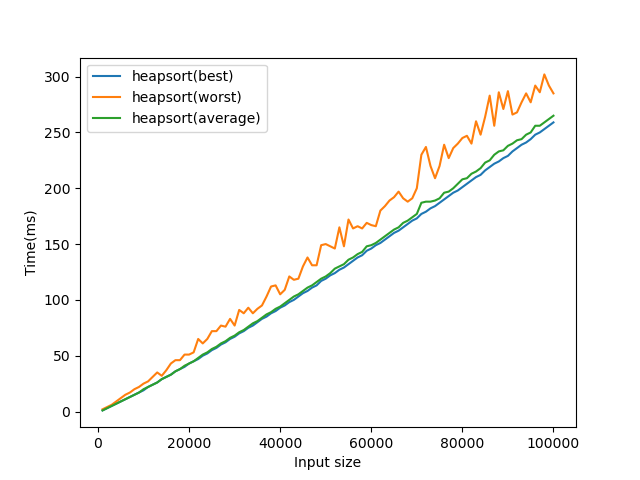
I'll leave you, as in the other sorting articles, with a plot of a simple benchmark showing our analysis was on point:

Conclusion

We have learned about heaps, a data structure whose main claim to fame is quickly providing access to the minimum of a collection of elements and utilized them to construct a theoretically optimal comparison based sorting algorithm.

Next time, we will explore how sorting could - in some cases - be improved even further by combining all of our knowledge with some assumptions about the input whilst allowing more than just comparisons.