Introduction to Algorithm Analysis (3): Quicksort

(Here is Part1 and Part2)

Whilst evaluating its utility we will find our toolbox to be insufficient and extend it with a new kind of analysis.

Quicksort

So what is quicksort? Like BubbleSort, it is a generic, comparison based sorting algorithm. Unlike BubbleSort, since its inception in 1959 by Tony Hoare - one of the most influential computer scientist still alive - it has seen considerable usage in real life, large scale software systems. Even today, the official Java reference implementation uses it in its library, the standard C function qsort is named after it and both the Rust and C++ standard libraries utilize improved variations.

Such an influential algorithm with "quick" in its very name, widespread use and even adoption by multiple languages known for their favorable performance characteristics must possess amazing qualities and incredibly low asymptotic complexity, right? Well, let's find out!

How does it work?

Quicksort utilizes a more general paradigm known as divide and conquer. Faced with a task so complex that it seems insurmountable, we break it down into more and more successively smaller pieces, until the problem becomes trivial or dissipates in its entirety.

Sorting a list of 8 elements is hard. We don't want to do that. Instead, sorting two lists of 4 elements each seems much better. Still too difficult so, so how about making that 4 lists of 2 elements? That seems easy enough. If we can get it down to just one element, our problem disappears, as such lists are - of course - always ordered perfectly.

Breaking a list into perfectly balanced sublists that are themselves ordered is, however, not exactly trivial and if we tried that, we would likely have to add an additional step to merge the parts together. Whilst possible, that is a different algorithm. Quicksort is simpler, at the cost of guaranteed balance: We choose one element to use as a pivot and reorder elements, such that all smaller than the pivot appear before all those larger than it. That is, given a list like this

[4,3,8,5,2]

and using 4 as the pivot element, we produce

[2,3] 4 [8,5]

or alternatively

[3,2] 4 [8,5]

or

[2,3] 4 [5,8]

You get the idea. The exact order inside the two new sublists does not matter, all we care about is the fact that everything on the left side is smaller than everything on the right side. Having done that, we repeat the same process on all sublists. That is the complete process. Expressed in simplified pseudocode:

if begin<end:
    partition_point = partition(begin, end, pivot)
	quicksort(begin,partition_point)
	quicksort(partition_point+1,end)

Partitioning can, of course, be done in a variety of ways. A popular choice used throughout this article is the original, known simply as Hoare partition:

pivot = chose_pivot()

while begin < end:

	while element_at(begin) < pivot:
		begin = begin + 1
		
	while element_at(end) > pivot:
		end = end - 1
	
	if begin<end:
		swap elements at begin and end

swap pivot to end

We search for the first element bigger than our pivot and the last smaller one. We swap the two and repeat our search further inward. Once the two positions cross, we found our partition point, with the swaps assuring everything left remains smaller, everything right remains bigger.

You might have noticed, that I have left open how exactly the pivot is chosen, as that constitutes yet another customization point.

Whilst there are arguably better ways to do it - yielding stronger guarantees - for simplicities sake, we will continue to arbitrarily chose the first element as our pivot.

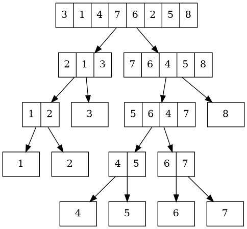
Applying this process to a simple example yields a recursive execution corresponding to this tree(notice how the leaves are ordered ascendingly):

Worst Case

Equipped with this understanding, we can finally put our newfound skills - acquired in the previous article - to the test. What is the best and worst case asymptotic complexity?

Counting operations might seem more complicated this time around, as the recursive calls obscure matters, but it is still doable. The trick is to visualize the call tree and argue based on its shape and the amount of operations performed on each layer.

All the real work happens inside partition and, as a swap happens only based on a comparison, it suffices to look at comparisons to obtain an upper bound.

At each layer of the call tree, partition is called for each sublist, comparing each of its elements to the chosen pivot exactly once. As every single one of the n elements is contained in one of those sublist, the sum total of elements processed is exactly n. So, independent of the distribution among sublists, we execute n comparisons per layer and our task simplifies to determining the height of said tree.

The smallest binary tree is a perfectly balanced one, as seen here:

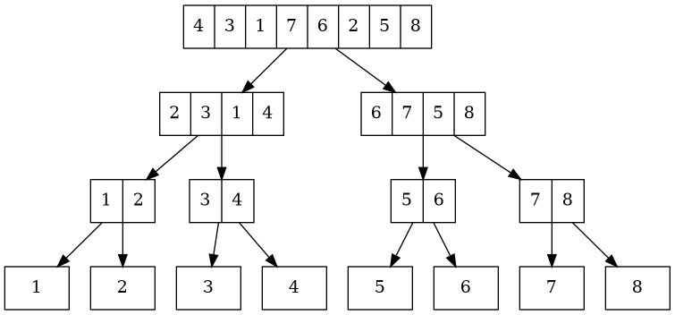
With each call, the list size gets cut in half, which happens until it is one. To determine the height, we have to answer the question of how often can we divide n by 2? That is

n/2/2/2/2/... = 1

This implies we have to solve

n/2^x = 1
n = 2^x
=> x = log2(n)

As such, our best case complexity is O(n * log(n))!

What is the worst case? The highest tree is unbalanced, tilted entirely to one side:

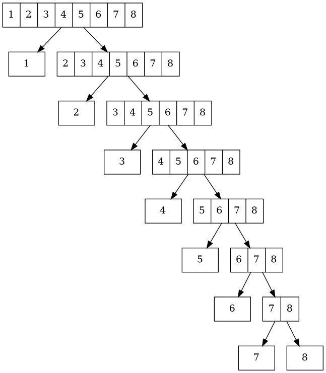
Hitting the smallest element as pivot yields sublists of 1 and n-1, so the height is bounded by how often we can subtract 1, which is n.
Granted, I lied when I claimed we compare all elements at each layer. We can save the comparisons for sublists of size 1. Still, as we realized when analyzing BubbleSort, n+n-1+n-2+n-3... is still quadratic.

As such, the worst case complexity is O(n^2)!

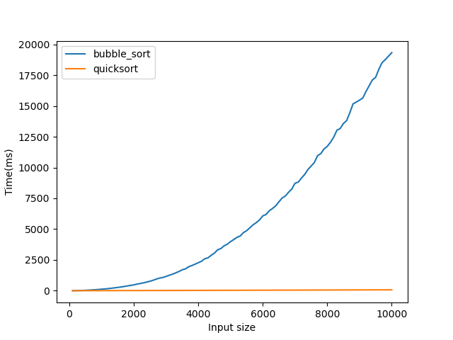
Despite its name, quicksort seems no better - even worse - than a simplistic bubblesort? That can't be true, can it? A wise developer once said: if in doubt, measure. So that is what I did:

Why?

What is going on here!? The worst case is equal, the best case is worse, but the real life performance is off the charts? Was our analysis erroneous? Not really. Let's zoom in a little:

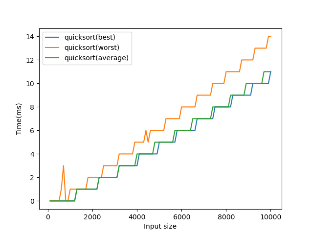
To generate this plot, I ran the algorithm for each size on 1000 different permutations and noted down the best, worst and average times. Notice how the lines for best and average overlap almost constantly? That tells us our worst case is exceedingly rare.

Average Case

The frequency of worst and best cases obviously matters. Yet, how do we analyze this? We have to think about that very frequency. Averaged over all possible permutations, what is the runtime of our sort?

With increasing n, the number of permutations grows rapidly (n!), whilst the number of worst case instances remains a constant and increasingly insignificant 2, which is highly unlikely to be hit. But what about all those cases in between? What happens if our pivot is the 2nd element? Or the 3rd? And so on?

It turns out the average is within O(n*log(n))! Proving that mathematically rigorous is quite involved and certainly outside the scope of an introductory article, but I shall provide a general sketch of one proof to convey the idea:

As we try to average over all possible permutations, choosing any one of them at random implies the desired position of our pivot element is a uniform random number between 1 and n. That is, each position is equally likely. Let's abuse that: Our pivot element is within the middle 50% exactly 50% of the time. Being pessimistic and overestimating our runtime, we can assume it to be the first element 50% of the time and the 25% position element in all other cases.

Using that assumption, we can describe the expected height of our call tree based on itself:

$$H(n) = H(n-1)/2 + H(3*n/4)/2 + 1$$

That is a lovely recurrence relation and an asymptotic bound for it can be computed: O(log n)
The statement made during worst case analysis still holds true. For each layer, we perform O(n) work, which gives a bound of O(n*log(n)), equal to our best case!

Conclusion

Best and worst case alone do not necessarily tell the complete story. When analyzing an algorithm, it can prove beneficial or even required to look at what happens on average. If a worst case is sufficiently rare and you do not have real time requirements, it might be alright. Alternatively, you could try to detect the worst case and avert it by creating a hybrid algorithm that falls back to a safer - albeit less performant - alternative.